

到目前为止,尝试在 Latex 中重新创建此操作尚未成功:

我使用的代码是这样的:
 \documentclass[14pt]{extarticle}

 \usepackage{pgfplots}
 \usepackage{tikz}
 \usepackage{ifthen}

 \begin{document}

 \pgfplotsset{compat=1.14}
 \begin{center}
 \begin{tikzpicture}%[scale=1.5]
 \begin{axis}[
 width=\textwidth,
 xmin = -1, xmax = 1,
 ymin = 0, ymax = 3,
 domain = -1: 1,
 xlabel = $x$,
 ylabel = $y$,
 axis x line = center,
every axis x label/.append style = {below},
every axis y label/.append style = {left},
samples = 100,
xtick = {-1, 0, 1},
xticklabels = {$-1$, $0$, $1$},
declare function = {
  s(\x) = ifthenelse(\x < pi, 1, 0);
  s0(\x) = 0.5  + (2 / (pi * pi)) * (1-cos(pi)) * cos(deg(\x * pi));
  s1(\x) = s0(\x) + (2 / (pi * pi * 9)) * (1-cos((\x * pi * 3)) * cos(deg(\x * pi * 3));
  s2(\x) = s1(\x) + (2 / (pi * pi * 25)) * (1-cos((\x * pi * 5)) * cos(deg(\x * pi * 5));
  s3(\x) = s1(\x) + (2 / (pi * pi * 49)) * (1-cos((\x * pi * 7)) * cos(deg(\x * pi * 7));
}, ]
\addplot[ultra thick, black] {s(x)};
\addplot[thick, blue] {s0(x)};
\addplot[thick, red] {s1(x)};
\addplot[thick, orange] {s2(x)};
\addplot[thick, cyan] {s3(x)};
\legend{signal, $s_0$, $s_1$, $s_2$, $s_3$};
% labels
\draw[gray, dashed] (-1, 0) -- (-1, 2);
\draw[gray, dashed] (1, 0) -- (1, 2);
\end{axis}
\end{tikzpicture}
\end{center}


\end{document}
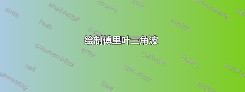
当前输出为:
 我的错误可能更多的是数学性质的而不是与 Latex 相关的,但如果有人能帮助我,我将不胜感激。
答案1
这里有两个主要问题,一个与有关pgfplots,一个与数学有关。正如我在评论中提到的,当谈到余弦函数的参数时,你有点前后矛盾。pgf假设输入以度为单位,因此当你输入弧度时,你应该将其转换为度。你在某些情况下会这样做,但不是所有情况。
您还可以通过添加选项来pgfplots假设三角函数的弧度。(比我在评论中提到的要好,因为后者也会影响 ylabel 等的旋转。)trig format plots=radaxistrig format plotstrig formats
数学问题是在 中s1,s2且s3有(1-cos((\x * pi * m)),应该是(1-cos(pi * m)),即否,\x*并且括号也是错误的。
下面的代码中还有一些其他更改,以使其更接近你的草图。我还定义了一个函数
sN(\N, \x) = (2 / (pi * pi * \N * \N)) * (1-cos(pi * \N)) * cos(\x * pi * \N);
减少代码重复并使其他函数定义更容易。

\documentclass[14pt]{extarticle}
\usepackage{pgfplots}
\pgfplotsset{compat=1.14}
\begin{document}
\begin{center}
\begin{tikzpicture}
\begin{axis}[
 width=\textwidth,height=0.5\textwidth,
 xmin = -1, xmax = 1,
 ymin = 0, ymax = 1.2, % changed from 3
 domain = -1: 1,
 xlabel = $x$,
 ylabel = $y$,
 hide y axis, % from your sketch you don't seem to want any y-axis
 axis x line = bottom, % changed from center
 samples = 101,
 xtick = {-1, 0, 1},
 trig format plots=rad, % added this, so pgfplots assumes radians for trig functions
 clip=false, % to avoid clipping half of the dashed lines
 declare function = {
   % signal function
   s = ifthenelse(\x<0, \x+1, -\x+1);
   % constant term
   s0 = 1/2;
   % generic function for term number N in the series
   sN(\N, \x) = (2 / (pi * pi * \N * \N)) * (1-cos(pi * \N)) * cos(\x * pi * \N);
   s1(\x) = s0  + sN(1,\x);
   s2(\x) = s1(\x) + sN(3,\x);
   s3(\x) = s2(\x) + sN(5,\x);
   s4(\x) = s3(\x) + sN(7,\x);
 }
]

\addplot[ultra thick, black, samples at={-1,0,1}] {s};
\addplot[thick, black] {s0};
\addplot[thick, blue] {s1(x)};
\addplot[thick, red] {s2(x)};
\addplot[thick, orange] {s3(x)};
\addplot[thick, cyan] {s4(x)};
\legend{signal, $s_0$, $s_1$, $s_2$, $s_3$, $s_4$};

% just a different method for making the vertical dashed lines
% yours works fine as well
\addplot [forget plot, ycomb, dashed, gray] coordinates {(-1,1.2)(1,1.2)};

\end{axis}
\end{tikzpicture}
\end{center}
\end{document}