

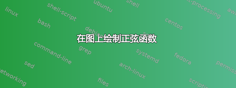
我试图在图表上绘制正弦(盒子中粒子的波函数)。预期结果是:

但是,目前的情况是这样的:

这是从以下代码中获得的:
% Diagram of a particle in 1D infinite potential well.
\newcommand{\vandbarrier}[1]{%
   \node at (#1, 1) {\scriptsize $V = \infty$};
   \node[scale = 0.5] at (#1, 0.5) {\textbf{(Barrier)}};%
}

\newcommand{\vabove}[1]{%
   \node[anchor = south] at (#1, 2) {\scriptsize $V = \infty$};%
}

\begin{tikzpicture}
\fill[mygray] % mygray is custom defined color.
    (0, 0) rectangle (2, 4)
    (4, 0) rectangle (6, 4);

\vandbarrier{1.0}
\vandbarrier{5.0}
\node[anchor = north] at (2, 0) {\scriptsize 0};
\node[anchor = north] at (4, 0) {\scriptsize $L$};
\node[anchor = north] at (6, 0) {\scriptsize $x$};

\draw[<->] (0, 0) to (6, 0);
\draw[->] (2, 0) to (2, 4);
\draw[->] (4, 0) to (4, 4);

\begin{axis}[
    %axis lines = none,
    xmin = 0, xmax = 3,
    ymin = 0, ymax =1,
    ]
    \addplot[domain = 0 : pi]{sin(deg(x))};
\end{axis}
\end{tikzpicture}
绘制上述图形最简单的方法是什么?
更具体地说:如果您能提供一些有关缩放和平移的语法和选项的帮助,axis我们将不胜感激。addplot
答案1
像第一个给定图像的选项结果,以及其他答案中显示的代码的一些很好的摘要。
结果:

梅威瑟:
\documentclass[tikz,border=0pt]{standalone}
\usetikzlibrary{arrows.meta}
\usepackage[scaled]{helvet}
\usepackage{stix}
\begin{document}
\definecolor{bg}{HTML}{FFE4C7}
\pagecolor{bg}
    \begin{tikzpicture}[
        %Environment cfg
        >={Stealth[length=9pt,inset=0]},
        font=\sffamily
    ]
    \def\L{3}
    \def\Deep{6}
    \def\Border{0.8}
    \def\h1{0.6}
    \def\Amp{1}
    \def\Spread{1.2}

    \fill[black!40]
    (0,0)
        |- ++(\L,-\Deep)
        |- ++(\Border,\Deep)
        |- ++(-\L -2*\Border,-\Deep -\Border)
        |- cycle;
    \draw[line width=2pt, <->]
    (0,0)++(0,\h1)
        node[anchor=south](T1){$\mathsf{\infty}$}
        |- ++(\L,-\Deep-\h1) -- ++(0,\Deep+\h1)
        node[anchor=south](T2){$\mathsf{\infty}$};
    \draw[thick,<->]
        (0,-\Deep+0.5) -- ++ (\L,0) node[midway,fill=bg]{L = \L};

    \foreach \n in {1,2,3,4}{
    \draw[very thick]
        (-0.4,-\Deep+\n*\Spread) node{n=\n}
        plot[
            variable=\x,
            domain=0:\L,
            smooth
        ]({\x},{-\Deep+\n*\Spread+0.4*sin(\x*360*0.5*\n/\L)});
    }
    \end{tikzpicture}
\end{document}
答案2
你不一定需要 pgfplots 来实现这一点。编辑:错误已修复,非常感谢 Max!
\documentclass[tikz,border=3.14mm]{standalone}
\begin{document}
\definecolor{mygray}{RGB}{127,127,127}
\newcommand{\vandbarrier}[1]{%
   \node at (#1, 1) {\scriptsize $V = \infty$};
   \node[scale = 0.5] at (#1, 0.5) {\textbf{(Barrier)}};%
}

\newcommand{\vabove}[1]{%
   \node[anchor = south] at (#1, 2) {\scriptsize $V = \infty$};%
}

\begin{tikzpicture}
\fill[mygray] % mygray is custom defined color.
    (0, 0) rectangle (2, 4)
    (4, 0) rectangle (6, 4);

\vandbarrier{1.0}
\vandbarrier{5.0}
\node[anchor = north] at (2, 0) {\scriptsize 0};
\node[anchor = north] at (4, 0) {\scriptsize $L$};
\node[anchor = north] at (6, 0) {\scriptsize $x$};

\draw[latex-latex,very thick] (0, 0) to (6, 0);
\draw[-latex,very thick] (2, 0) to (2, 4);
\draw[-latex,very thick] (4, 0) to (4, 4);

\draw[blue,thick] plot[variable=\x,domain=-1:1,smooth] ({\x+3},{1+0.4*cos(\x*120)});
\draw[blue,thick] plot[variable=\x,domain=-1:1,smooth] ({\x+3},{2-0.4*sin(\x*180)});
\draw[blue,thick] plot[variable=\x,domain=-1:1,smooth] ({\x+3},{3-0.4*cos(\x*270)});
\end{tikzpicture}
\end{document}

答案3
@marmot 答案的另一种选择是使用sin和cos路径命令:

\documentclass[tikz,margin=2mm]{standalone}

\definecolor{mygray}{gray}{0.4}

\begin{document}
% Diagram of a particle in 1D infinite potential well.
\newcommand{\vandbarrier}[1]{%
   \node at (#1, 1) {\scriptsize $V = \infty$};
   \node[scale = 0.5] at (#1, 0.5) {\textbf{(Barrier)}};%
}

\newcommand{\vabove}[1]{%
   \node[anchor = south] at (#1, 2) {\scriptsize $V = \infty$};%
}

\begin{tikzpicture}
\fill[mygray] % mygray is custom defined color.
    (0, 0) rectangle (2, 4)
    (4, 0) rectangle (6, 4);

\vandbarrier{1.0}
\vandbarrier{5.0}
\node[anchor = north] at (2, 0) {\scriptsize 0};
\node[anchor = north] at (4, 0) {\scriptsize $L$};
\node[anchor = north] at (6, 0) {\scriptsize $x$};

\draw[<->] (0, 0) to (6, 0);
\draw[->] (2, 0) to (2, 4);
\draw[->] (4, 0) to (4, 4);

\pgfmathsetmacro\amplitude{0.5}

\draw (2,1) sin ++(1,\amplitude) cos ++(1,-\amplitude);
\draw (2,2) sin ++(1/2,\amplitude) cos ++(1/2,-\amplitude) sin ++(1/2,-\amplitude) cos ++(1/2,\amplitude);
\draw (2,3) sin ++(1/3,\amplitude) cos ++(1/3,-\amplitude) sin ++(1/3,-\amplitude) cos ++(1/3,\amplitude) sin ++(1/3,\amplitude) cos ++(1/3,-\amplitude);

\end{tikzpicture}
\end{document}
编辑
只是为了好玩,同样的解决方案,但现在使用嵌套\foreach来绘制任意数量的、频率不断增加的波:

\documentclass[tikz,margin=2mm]{standalone}

\definecolor{mygray}{gray}{0.4}

\begin{document}
% Diagram of a particle in 1D infinite potential well.
\newcommand{\vandbarrier}[1]{%
   \node at (#1, 1) {\scriptsize $V = \infty$};
   \node[scale = 0.5] at (#1, 0.5) {\textbf{(Barrier)}};%
}

\newcommand{\vabove}[1]{%
   \node[anchor = south] at (#1, 2) {\scriptsize $V = \infty$};%
}

\begin{tikzpicture}
\fill[mygray] % mygray is custom defined color.
    (0, 0) rectangle (2, 4)
    (4, 0) rectangle (6, 4);

\vandbarrier{1.0}
\vandbarrier{5.0}
\node[anchor = north] at (2, 0) {\scriptsize 0};
\node[anchor = north] at (4, 0) {\scriptsize $L$};
\node[anchor = north] at (6, 0) {\scriptsize $x$};

\draw[<->] (0, 0) to (6, 0);
\draw[->] (2, 0) to (2, 4);
\draw[->] (4, 0) to (4, 4);

\pgfmathsetmacro\amplitude{0.2}

\foreach \i in {1,...,8}{
    \draw[blue] (2,{(\i-1)*\amplitude*2.2+1.1*\amplitude}) foreach \j [evaluate=\j as \dir using {(-1)^\j}]in {1,...,\i}{
        sin ++(1/\i,-1*\dir*\amplitude) cos ++(1/\i,\dir*\amplitude)
    };
}
%\draw (2,1) sin ++(1/1,\amplitude) cos ++(1/1,-\amplitude);
%\draw (2,2) sin ++(1/2,\amplitude) cos ++(1/2,-\amplitude) sin ++(1/2,-\amplitude) cos ++(1/2,\amplitude);
%\draw (2,3) sin ++(1/3,\amplitude) cos ++(1/3,-\amplitude) sin ++(1/3,-\amplitude) cos ++(1/3,\amplitude) sin ++(1/3,\amplitude) cos ++(1/3,-\amplitude);

\end{tikzpicture}
\end{document}