

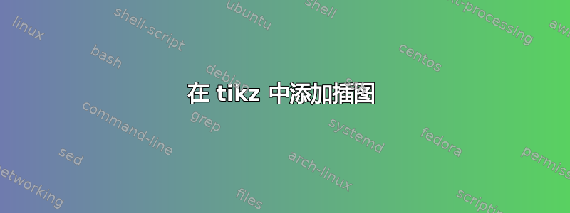
是否可以像插图样式的图形一样绘制,但仅使用 tikz ? 显然,我试图通过聚焦于方案的特定区域来使用缩放效果,但我想要实现的是:
- 在插图中,我想在红点中显示全局轮廓的一部分,然后添加相同轮廓的形状,但在箭头末端的点。因此,这两个轮廓只需要出现在放大的区域中,而不是整个图片中:这就是我在这里挣扎的主要原因
您认为怎样才有可能实现这一目标?
谢谢您的意见,
此致。
代码 :
\documentclass{article}
\usepackage[utf8]{inputenc}

%%%%%%%%MATHS%%%%%%%%%%%%%
\usepackage{amsmath}
\usepackage{amsfonts}
\usepackage{color} %red, green, blue, yellow, cyan, magenta, black, white

%%%%%%%%GEOMETRIE%%%%%%%%%%%
\usepackage{geometry}
\usepackage{layout}


%%%AXIS%%%%
\usepackage{pgfplots}
\pgfplotsset{compat=newest}

%%%%%%%%SECTIONS/AGENCEMENT%%%
\usepackage{pgf, tikz, adjustbox}
\usepgfplotslibrary{fillbetween}
\usetikzlibrary{calc}
\usetikzlibrary{spy}
\usetikzlibrary{patterns, matrix, positioning}
\usetikzlibrary{arrows.meta,
                patterns.meta
                }

\usepackage[framemethod=tikz]{mdframed} % breakable frames and coloured boxes
\usetikzlibrary{decorations.pathmorphing}
%%%%%%%%GAUSSIAN%%%%%%%%%%%%
\pgfmathdeclarefunction{gauss}{1}{%
    \pgfmathparse{3*exp(-(#1/2.5)^2)}
}

\begin{document}

\begin{figure}[h]
\centering
\begin{tikzpicture}[spy using outlines,
dot/.style = {circle, fill, inner sep=2.0pt, node contents={}},
  scale = 1,
  s/.style={shift=(0:9)}]
\fill [cyan!20]
          plot[domain= -4:13, samples=100] (\x, {gauss(\x)+gauss(\x-9})
       |- (-4,0)
       -| cycle;
\filldraw[fill=pink!20, thick]
          plot[domain=-4:13, samples=100] (\x, {gauss(\x)+gauss(\x-9)})
       -- plot[domain=13:-4, samples=100] (\x, {gauss(\x)+gauss(\x-9)+0.2})
       -- cycle;
\path[fill=cyan!20] (-0.5,-2) -- (-0.5,0) -- (0.5,0) -- (0.5,-2) -- (-0.5,-2);
\path[fill=cyan!20] (8.5,-2) -- (8.5,0) -- (9.5,0) -- (9.5,-2) -- (8.5,-2);
\draw[black,thick] (0.5,-2) -- (0.5,0) -- (8.5,0) -- (8.5,-2);
\draw[black,thick] (-0.5,-2) -- (-0.5,0) -- (-4,0);
\draw[black,thick] (9.5,-2) -- (9.5,0) -- (13,0);
\draw[dashed,red, stealth-stealth, thick] (-0.5,-2.25) -- node[below,scale=0.75] {$e \sim 1 \ mm$} (0.5,-2.25);
\draw [yshift=-0.25cm, -latex](0,-1.5) -- node [fill=cyan!20,scale=0.75] {$Q_1$} (0,0);
\draw [yshift=-0.25cm, -latex](9,-1.5) -- node [fill=cyan!20,scale=0.75] {$Q_2$} (9,0);
\spy [blue,draw,height=3cm,width=7cm,magnification=2,connect spies] on (4.5,0.85) in node at (4.5,5);  % ZOOM EFFECT
\coordinate [red]  (A) at (4.5,0.45)  ;
\coordinate [red]  (B) at (4.5,1.35)  ;
\draw[dashed,-stealth,black!30!red,thick] (A) to  (B) ;
\path (4.5,0.45) node[black!30!red,dot] ;
\end{tikzpicture}
\end{figure}
\end{document}
图像 :

编辑
我正在尝试改进我以前的尝试,并考虑使用以下帖子中建议的混合解决方案:帖子1和帖子2 通过实现保存框功能并将两个不同的图表链接在一起
我仍然对此不满意:由于某种原因,我无法理解为上面第二张图片创建的节点的大小,我希望该节点位于第一个主图的中间,但没有成功做到这一点......
第二个代码:
\documentclass{article}
\usepackage[utf8]{inputenc}

%%%%%%%%MATHS%%%%%%%%%%%%%
\usepackage{amsmath}
\usepackage{amsfonts}

%%%%%%%%GEOMETRIE%%%%%%%%%%%
\usepackage{geometry}
\usepackage{layout}


%%%AXIS%%%%
\usepackage{pgfplots}
\pgfplotsset{compat=newest}

%%%%%%%%SECTIONS/AGENCEMENT%%%
\usepackage{pgf, tikz, adjustbox}
\usepgfplotslibrary{fillbetween}
\usetikzlibrary{calc}
\usetikzlibrary{spy}
\usetikzlibrary{patterns, matrix, positioning}
\usetikzlibrary{arrows.meta,
                patterns.meta
                }

\usepackage[framemethod=tikz]{mdframed} % breakable frames and coloured boxes
\usetikzlibrary{decorations.pathmorphing}
%%%%%%%%GAUSSIAN%%%%%%%%%%%%
\pgfmathdeclarefunction{gauss}{1}{%
    \pgfmathparse{3*exp(-(#1/2.5)^2)}
}
\pgfmathdeclarefunction{gaussquatre}{1}{%
    \pgfmathparse{3*exp(-(#1/1.5)^2)}
}

%%%%% DOCUMENT%%%%%%
\begin{document}


\newsavebox\Graphone
\sbox\Graphone{\begin{tikzpicture}[spy using outlines,
dot/.style = {circle, fill, inner sep=1.5pt, node contents={}},
  scale = 1,
  s/.style={shift=(0:9)}]
\fill [cyan!20]
          plot[domain= -4:13, samples=100] (\x, {gauss(\x)+gauss(\x-9})
       |- (-4,0)
       -| cycle;
\filldraw[fill=pink!20, thick]
          plot[domain=-4:13, samples=100] (\x, {gauss(\x)+gauss(\x-9)})
       -- plot[domain=13:-4, samples=100] (\x, {gauss(\x)+gauss(\x-9)+0.2})
       -- cycle;
\path[fill=cyan!20] (-0.5,-2) -- (-0.5,0) -- (0.5,0) -- (0.5,-2) -- (-0.5,-2);
\path[fill=cyan!20] (8.5,-2) -- (8.5,0) -- (9.5,0) -- (9.5,-2) -- (8.5,-2);
\draw[black,thick] (0.5,-2) -- (0.5,0) -- (8.5,0) -- (8.5,-2);
\draw[black,thick] (-0.5,-2) -- (-0.5,0) -- (-4,0);
\draw[black,thick] (9.5,-2) -- (9.5,0) -- (13,0);
\draw[dashed,red, stealth-stealth, thick] (-0.5,-2.25) -- node[below,scale=0.75] {$e \sim 1 \ mm$} (0.5,-2.25);
\draw [yshift=-0.25cm, -latex](0,-1.5) -- node [fill=cyan!20,scale=0.75] {$Q_1$} (0,0);
\draw [yshift=-0.25cm, -latex](9,-1.5) -- node [fill=cyan!20,scale=0.75] {$Q_2$} (9,0);
\draw[black, pattern = checkerboard] (-0.5,-.5) -- (-0.5,0) -- (-4,0) -- (-4,-.5) -- cycle;
\draw[black, pattern = checkerboard] (9.5,-.5) -- (9.5,0) -- (13,0) -- (13,-.5) -- cycle;
\draw[black, pattern = checkerboard] (0.5,-.5) -- (0.5,0) -- (8.5,0) -- (8.5,-.5) -- cycle;
\end{tikzpicture}}

\newsavebox\Graphbis
\sbox\Graphbis{\begin{tikzpicture}[spy using outlines,
dot/.style = {circle, fill, inner sep=1.5pt, node contents={}},
  scale = 1,
  ]
\fill [cyan!20]
          plot[domain= 2.5:6.5, samples=100] (\x, {gauss(\x)+gauss(\x-9})
       |- (-4,0)
       -| cycle;
\filldraw[fill=pink!20, thin]
          plot[domain=2.5:6.5, samples=100] (\x, {gauss(\x)+gauss(\x-9)})
       -- plot[domain=6.5:2.5, samples=100] (\x, {gauss(\x)+gauss(\x-9)+0.1})
       -- cycle;
\filldraw[fill=pink!20, thin]
          plot[domain=2.5:6.5, samples=100] (\x, {gaussquatre(\x)+gaussquatre(\x-9)+1})
       -- plot[domain=6.5:2.5, samples=100] (\x, {gaussquatre(\x)+gaussquatre(\x-9)+1.1})
       -- cycle;
\coordinate [red]  (A) at (4.5,0.3)  ;
\coordinate [red]  (B) at (4.5,1.1)  ;
\draw[dashed,-stealth,black!30!red,thin] (A) to  (B) ;
\path (4.5,0.285) node[black!30!red,dot] ;
\end{tikzpicture}}

%%%%%%FIGURE
\begin{figure}[h]
\centering
\begin{tikzpicture}
\node(a){\usebox{\Graphone}};
\node(b)[inner sep=0pt,above = 0.5cm of a] {\phantom{\usebox{\Graphbis}}};
\node(c)[draw,minimum size=0.5cm, at=(a)]{};
\begin{scope}[thin,blue!40]
\draw(c.north east) -- (b.south east);
\draw(c.north west) -- (b.south west);
\end{scope}
\node [at=(b),inner sep=0pt,above = 0.5cm of a] {\usebox{\Graphbis}};
\end{tikzpicture}
\end{figure}

\end{document}
图片 :

答案1
参照 Jasper Habicht 在帖子 2 中的回答,我们可以使用pic。我使用\clip和transform canvas。我使用math库来声明比例。使用比例 ( \e),坐标被修改。在红点 (4.5,0) 上方找到的偏移量乘以(\e - 1)
\documentclass[border=3cm]{standalone}
%%%AXIS%%%%
\usepackage{pgfplots}
\pgfplotsset{compat=newest}
%%%%%%%%SECTIONS/AGENCEMENT%%%
\usetikzlibrary {math}%<-- added
\usetikzlibrary{patterns}
%%%%%%%%GAUSSIAN%%%%%%%%%%%%
\pgfmathdeclarefunction{gauss}{1}{%
    \pgfmathparse{3*exp(-(#1/2.5)^2)}
}
\pgfmathdeclarefunction{gaussquatre}{1}{%
    \pgfmathparse{3*exp(-(#1/1.5)^2)}
}

%%%%% DOCUMENT%%%%%%
\begin{document}
\tikzset{
  dot/.style = {circle, fill, inner sep=2.0pt, node contents={}},
  Graphone/.pic={
    \fill [cyan!20]
          plot[domain= -4:13, samples=100] (\x, {gauss(\x)+gauss(\x-9})
      |- (-4,0)
      -| cycle;
    \filldraw[fill=pink!20, thick]
              plot[domain=-4:13, samples=100] (\x, {gauss(\x)+gauss(\x-9)})
          -- plot[domain=13:-4, samples=100] (\x, {gauss(\x)+gauss(\x-9)+0.2})
          -- cycle;
    \path[fill=cyan!20] (-0.5,-2) -- (-0.5,0) -- (0.5,0) -- (0.5,-2) -- (-0.5,-2);
    \path[fill=cyan!20] (8.5,-2) -- (8.5,0) -- (9.5,0) -- (9.5,-2) -- (8.5,-2);
    \draw[black,thick] (0.5,-2) -- (0.5,0) -- (8.5,0) -- (8.5,-2);
    \draw[black,thick] (-0.5,-2) -- (-0.5,0) -- (-4,0);
    \draw[black,thick] (9.5,-2) -- (9.5,0) -- (13,0);
    \draw[dashed,red, stealth-stealth, thick] (-0.5,-2.25) -- node[below,scale=0.75] {$e \sim 1 \ mm$} (0.5,-2.25);
    \draw [yshift=-0.25cm, -latex](0,-1.5) -- node [fill=cyan!20,scale=0.75] {$Q_1$} (0,0);
    \draw [yshift=-0.25cm, -latex](9,-1.5) -- node [fill=cyan!20,scale=0.75] {$Q_2$} (9,0);
    \coordinate [red]  (A) at (4.5,0.45)  ;
    \coordinate [red]  (B) at (4.5,1.35)  ;
    \draw[dashed,-stealth,black!30!red,thick] (A) to  (B) ;
    \path (4.5,0.45) node[black!30!red,dot] ;
    },
  Graphbis/.pic={
    \fill [cyan!20]
          plot[domain= 2.5:6.5, samples=100] (\x, {gauss(\x)+gauss(\x-9})
      |- (-4,0)
      -| cycle;
    \filldraw[fill=pink!20, thin]
              plot[domain=2.5:6.5, samples=100] (\x, {gauss(\x)+gauss(\x-9)})
          -- plot[domain=6.5:2.5, samples=100] (\x, {gauss(\x)+gauss(\x-9)+0.1})
          -- cycle;
    \filldraw[fill=pink!20, thin]
              plot[domain=2.5:6.5, samples=100] (\x, {gaussquatre(\x)+gaussquatre(\x-9)+1})
          -- plot[domain=6.5:2.5, samples=100] (\x, {gaussquatre(\x)+gaussquatre(\x-9)+1.1})
      -- cycle;
    \coordinate [red]  (A) at (4.5,0.3)  ;
    \coordinate [red]  (B) at (4.5,1.1)  ;
    \draw[dashed,-stealth,black!30!red,thin] (A) to  (B) ;
    \path (4.5,0.285) node[black!30!red,dot] ;
  }
}
\tikzmath{
  real \e;
  \e = 1.25;  % scale
}
\begin{tikzpicture}
  \draw(0,0) grid (10,5);%<-- comment in the final document
  \pic (one) at (0,0) {Graphone};
  \draw [blue](2,0) rectangle(7,2);
  \begin{scope}[transform canvas={xshift=-4.5cm*(\e-1),yshift=3cm,scale=\e}]
    \clip (2,0) rectangle(7,2);
    \pic (one) at (0,0) {Graphone};
    \draw [red](0,0)--(10,2);% other code
  \end{scope}
\end{tikzpicture}

\end{document}

编辑:我会尽力解释
当 scale=2 时,坐标也乘以 2
\begin{scope}[transform canvas={yshift=3cm,scale=2}]

我们xshift=-4.5cm*(2-1)向左移动到坐标点 (4.5,0.5) 上方

对于图单和图二的联系,我对 做了一些修改shift={(4.5,0),在图单中加入了配位变量 (xone,yone) 和 (xbis,ybis)。
编辑2:添加shorten >=6pt和pos=0.5
\documentclass[border=5cm]{standalone}
%%%AXIS%%%%
\usepackage{pgfplots}
\pgfplotsset{compat=newest}
%%%%%%%%SECTIONS/AGENCEMENT%%%
\usetikzlibrary{patterns}
%%%%%%%%GAUSSIAN%%%%%%%%%%%%
\pgfmathdeclarefunction{gauss}{1}{%
    \pgfmathparse{3*exp(-(#1/2.5)^2)}
}
\pgfmathdeclarefunction{gaussquatre}{1}{%
    \pgfmathparse{3*exp(-(#1/1.5)^2)}
}
%%%%% DOCUMENT%%%%%%
\begin{document}
% \tikzset{
%   dot/.style = {circle, fill, inner sep=2.0pt, node contents={}},
% }
% \begin{tikzpicture}
%   \draw(0,0) grid (10,5);
%   \path (4.5,0.45) node[name=A,black!30!red,dot];
%   \path (2,0) node[name=B,black!30!red,dot];
%   \draw (A)--(B);
%   \begin{scope}[transform canvas={yshift=3cm,scale=2}]
%     \path (4.5,0.45) node[name=A,black!30!red,dot];
%     \path (2,0) node[name=B,black!30!red,dot];
%     \draw[red](A)--(B);
%   \end{scope}
% \end{tikzpicture}

% \begin{tikzpicture}
%   \draw(0,0) grid (10,5);
%   \path (4.5,0.45) node[name=A,black!30!red,dot];
%   \path (2,0) node[name=B,black!30!red,dot];
%   \draw (A)--(B);
%   \begin{scope}[transform canvas={xshift=-4.5cm*(2-1),yshift=3cm,scale=2}]
%     \path (4.5,0.45) node[name=A,black!30!red,dot];
%     \path (2,0) node[name=B,black!30!red,dot];
%     \draw[red](A)--(B);
%   \end{scope}
% \end{tikzpicture}

\tikzset{
dot/.style = {circle, fill, inner sep=2.0pt, node contents={}},
Graphone/.pic={
    \fill [cyan!20]
        plot[domain= -4:13, samples=100] (\x, {gauss(\x)+gauss(\x-9})
    |- (-4,0)
    -| cycle;
    \filldraw[fill=pink!20, thick]
            plot[domain=-4:13, samples=100] (\x, {gauss(\x)+gauss(\x-9)})
        -- plot[domain=13:-4, samples=100] (\x, {gauss(\x)+gauss(\x-9)+0.2})
        -- cycle;
    \path[fill=cyan!20] (-0.5,-2) -- (-0.5,0) -- (0.5,0) -- (0.5,-2) -- (-0.5,-2);
    \path[fill=cyan!20] (8.5,-2) -- (8.5,0) -- (9.5,0) -- (9.5,-2) -- (8.5,-2);
    \draw[black,thick] (0.5,-2) -- (0.5,0) -- (8.5,0) -- (8.5,-2);
    \draw[black,thick] (-0.5,-2) -- (-0.5,0) -- (-4,0);
    \draw[black,thick] (9.5,-2) -- (9.5,0) -- (13,0);
    \draw[dashed,red, stealth-stealth, thick] (-0.5,-2.25) -- node[below,pos=0.5,scale=0.75] {$e \sim 1 \ mm$} (0.5,-2.25);
    \draw [yshift=-0.25cm,-latex,shorten >=6pt](0,-1.5) -- node [fill=cyan!20,scale=0.75] {$Q_1$} (0,0);
    \draw [yshift=-0.25cm,-latex,shorten >=6pt](9,-1.5) -- node [fill=cyan!20,scale=0.75] {$Q_2$} (9,0);
    \coordinate [red]  (A) at (4.5,0.45)  ;
    \coordinate [red]  (B) at (4.5,1.35)  ;
    \draw[dashed,-stealth,black!30!red,thick] (A) to  (B) ;
    \path (4.5,0.45) node[black!30!red,dot];
    },
}

\begin{tikzpicture}[declare function={%
    s = 1.5;% scale
    ydecal=4cm;% offset of the clip
}]
\draw(0,0) grid (10,5);%<-- comment in the final document
\pic (A) at (0,0) {Graphone};
\draw [blue](2,0) rectangle(7,2);
%%%%%%%%%  clip and tranlate
\begin{scope}[transform canvas={xshift=-4.5cm*(s-1),yshift=ydecal,scale=s}]
    \clip (2,0)rectangle(7,2);
    \pic (B) at (0,0) {Graphone};
    % add code
    \filldraw[fill=pink!20, thin]
    plot[domain=2.5:6.5, samples=100] (\x, {gaussquatre(\x)+gaussquatre(\x-9)+1})-- plot[domain=6.5:2.5, samples=100] (\x, {gaussquatre(\x)+gaussquatre(\x-9)+1.1});
\end{scope}
%%%%%   change the repere
\begin{scope}[shift={(4.5,0)},
    declare function={%
    xone=-2.5;% offset of the start of the arrow relative to the red point
    yone=2;
    xbis=-2.5;
    ybis=0;
}]
    \draw[->,very thick](xone,yone)--(xbis*s,ybis*s+ydecal);
\end{scope}
\end{tikzpicture}
\end{document}
