

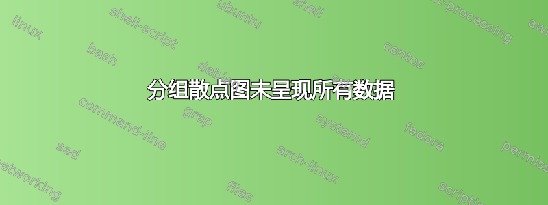
我有两个数据文件需要绘制在两个图中,我使用 pgfplots 中的 groupplots 包进行绘制。问题是文件中的数据并未全部绘制出来。我尝试更改和列hxe.dat的值,但仍然只呈现了三个标记。有人能帮帮我吗?我使用的代码如下。Blue-1CBlue-AC
\documentclass{article}
\usepackage{geometry}
\usepackage{graphicx} % Required for inserting images
\usepackage{pgfplots, filecontents}
\pgfplotsset{compat=1.10, width=20cm}
\usepgfplotslibrary{groupplots}
\usepgfplotslibrary{colorbrewer}
\usetikzlibrary{plotmarks}

\begin{filecontents*}{hxe.dat}
Method Red-1C Red-AC Blue-1C Blue-AC
Square 2.37 77.38 5.97 67.88
Triangle 1.48 77.96 5.98 70.23
Diamond 2.29 79.07 5.98 69.57
HDiamond 2.83 74.17 6.04 61.87
Circle 2.03 76.29 6.38 63.60
HCircle 2.29 78.68 6.23 64.97
HSquare 1.71 75.48 6.23 64.28
\end{filecontents*}

\begin{filecontents*}{bce.dat}
Method Red-1C Red-AC Blue-1C Blue-AC Vi-X Vi-Y
Square 2.37 77.38 8.75 75.56 5.97 67.88
Triangle 1.48 77.96 10.93 76.62 5.98 70.23
Diamond 2.29 79.07 10.06 77.78 5.98 69.57
HDiamond 2.83 74.17 9.42 72.78 6.04 61.87
Circle 2.03 76.29 10.15 76.50 6.38 63.60
HCircle 2.29 78.68 11.04 78.60 6.23 64.97
HSquare 1.71 75.48 10.63 74.45 6.23 64.28
\end{filecontents*}

\title{TestForGroupPlot}
\author{Satwik Srivastava (M21MA006)}
\date{March 2023}

\begin{document}

\maketitle


\begin{figure*}[t]
\centering
% \resizebox{0.95\textwidth}{!}{
\begin{tikzpicture}
\begin{groupplot}[
    group style={group size= 2 by 1, horizontal sep=4em,},height=8cm,width=8cm,
    xlabel={SoE},
    ylabel={AUROC},
    legend style={
        at={(-0.1,-0.2)},
        anchor=north,
        legend columns=7
    },
    ymajorgrids=true,
    xmajorgrids=true,
    xmin=1.0,
    xmax=14.0,
    ymin=65.0,
    ymax=85.0,
    yminorgrids = true,
    minor grid style=loosely dotted,
    scatter/classes={
        Diamond={mark=diamond*},
        HDiamond={mark=o},
        Square={mark=square*},
        Triangle={mark=triangle*},
        Circle={mark=*},
        HCircle={mark=square},
        HSquare={mark=x}
    },
    % only marks,
    scatter,
    scatter src=explicit symbolic,
    % axis background/.style={fill=BG!5}
]

\nextgroupplot[title=(a), scatter, only marks, mark size=2.5pt]
\addplot [
    color=black,
]
table[
    x=Red-1C,
    y=Red-AC,
    meta=Method
]
{bce.dat}; \label{bce1}


\addplot [
    color=blue,
]
table[
    x=Blue-1C,
    y=Blue-AC,
    meta=Method
]
{bce.dat}; \label{bce2}

% \begin{scope}[on background layer]
\fill[green,opacity=0.20] ({rel axis cs:0,1}) rectangle ({rel axis cs:0.25,0.6});
\fill[red,opacity=0.20] ({rel axis cs:1,0.5}) rectangle ({rel axis cs:0.25,0});
% \end{scope}

\nextgroupplot[title=(b), scatter, only marks, mark size=2.5pt,]
\addplot [
    color=black,
]
table[
    x=Red-1C,
    y=Red-AC,
    meta=Method
]
{hxe.dat}; \label{hxe1}

\addplot [
    color=violet,
    % opacity=0.4
]
table[
    x=Blue-1C,
    y=Blue-AC,
    meta=Method
]
{hxe.dat}; \label{hxe2}


% \begin{scope}[on background layer]
\fill[green,opacity=0.20] ({rel axis cs:0,1}) rectangle ({rel axis cs:0.25,0.6});
\fill[red,opacity=0.20] ({rel axis cs:1,0.5}) rectangle ({rel axis cs:0.25,0});
% \end{scope}

\legend{Resnet18, Resnet50, Densenet121, MobilenetV2, ShufflenetV2, Wideresnet50, EfficientnetB4}
\end{groupplot}

% Draw first "Legend" node using a left justified shortstack, position using relative axis coordinates
\node [draw,fill=white] at (rel axis cs: 0.208, -0.063) {\shortstack[l]{
\ref{bce1} Standard \\
\ref{bce2} CRM }};

\node [draw,fill=white] at (rel axis cs: 2.06, 0.75) {\shortstack[l]{
\ref{hxe1} BCE \\
\ref{hxe2} HXE}};

\end{tikzpicture} %}

\vspace{20pt}

\caption{Caption}
\label{fig:scatter}
\end{figure*}


\end{document}
以下是呈现的情节。

答案1
欢迎来到 TeX.SX!您声明了ymin = 65,因此小于该值的值将从图表区域中删除。减小此值,它们就会显示出来。
我建议进行以下改进:
- 将包含部分图例的节点移动到相关组图内。这样,您可以
rel axis cs更有效地与锚点一起使用来定位节点。 axis cs将彩色区域放置在背景平面上,并使用而不是使用来定义坐标rel axis cs。这样,你就可以使用X和是这里可能会派上用场的斧头。
\documentclass[border=10pt]{standalone}
\usepackage{pgfplots}
\pgfplotsset{compat=1.18, width=20cm}
\usepgfplotslibrary{groupplots}
\usetikzlibrary{backgrounds}

\begin{filecontents*}{hxe.dat}
Method Red-1C Red-AC Blue-1C Blue-AC
Square 2.37 77.38 5.97 67.88
Triangle 1.48 77.96 5.98 70.23
Diamond 2.29 79.07 5.98 69.57
HDiamond 2.83 74.17 6.04 61.87
Circle 2.03 76.29 6.38 63.60
HCircle 2.29 78.68 6.23 64.97
HSquare 1.71 75.48 6.23 64.28
\end{filecontents*}

\begin{filecontents*}{bce.dat}
Method Red-1C Red-AC Blue-1C Blue-AC Vi-X Vi-Y
Square 2.37 77.38 8.75 75.56 5.97 67.88
Triangle 1.48 77.96 10.93 76.62 5.98 70.23
Diamond 2.29 79.07 10.06 77.78 5.98 69.57
HDiamond 2.83 74.17 9.42 72.78 6.04 61.87
Circle 2.03 76.29 10.15 76.50 6.38 63.60
HCircle 2.29 78.68 11.04 78.60 6.23 64.97
HSquare 1.71 75.48 10.63 74.45 6.23 64.28
\end{filecontents*}

\begin{document}
\begin{tikzpicture}

\begin{groupplot}[
    group style={
        group size= 2 by 1,
        horizontal sep=4em,
    },
    height=8cm,
    width=8cm,
    xlabel={SoE},
    ylabel={AUROC},
    legend style={
        at={(-0.1,-0.2)},
        anchor=north,
        legend columns=7
    },
    ymajorgrids=true,
    xmajorgrids=true,
    xmin=1,
    xmax=14,
    ymin=60,
    ymax=85,
    yminorgrids = true,
    minor grid style=loosely dotted,
    scatter/classes={
        Diamond={mark=diamond*},
        HDiamond={mark=o},
        Square={mark=square*},
        Triangle={mark=triangle*},
        Circle={mark=*},
        HCircle={mark=square},
        HSquare={mark=x}
    },
    % only marks,
    scatter,
    scatter src=explicit symbolic,
    % axis background/.style={fill=BG!5}
]

\nextgroupplot[title=(a), scatter, only marks, mark size=2.5pt]
\addplot [
    color=black,
]
table[
    x=Red-1C,
    y=Red-AC,
    meta=Method
]
{bce.dat}; \label{bce1}

\addplot [
    color=blue,
]
table[
    x=Blue-1C,
    y=Blue-AC,
    meta=Method
]
{bce.dat}; \label{bce2}

\begin{scope}[on background layer]
\fill[green, opacity=0.2] (axis cs:1,77) rectangle (axis cs:4.25,85);
\fill[red, opacity=0.2] (axis cs:4.25,60) rectangle (axis cs:14,75);
\end{scope}

\node [draw, fill=white, anchor=south west] at ([shift={(5pt,5pt)}]rel axis cs:0,0) {\shortstack[l]{
\ref{bce1} Standard \\
\ref{bce2} CRM }};

\nextgroupplot[title=(b), scatter, only marks, mark size=2.5pt,]
\addplot [
    color=black,
]
table[
    x=Red-1C,
    y=Red-AC,
    meta=Method
]
{hxe.dat}; \label{hxe1}

\addplot [
    color=violet,
    % opacity=0.4
]
table[
    x=Blue-1C,
    y=Blue-AC,
    meta=Method
]
{hxe.dat}; \label{hxe2}

\begin{scope}[on background layer]
\fill[green, opacity=0.2] (axis cs:1,77) rectangle (axis cs:4.25,85);
\fill[red, opacity=0.2] (axis cs:4.25,60) rectangle (axis cs:14,75);
\end{scope}

\node [draw, fill=white, anchor=north east] at ([shift={(-5pt,-5pt)}]rel axis cs:1,1){\shortstack[l]{
\ref{hxe1} BCE \\
\ref{hxe2} HXE}};

\legend{Resnet18, Resnet50, Densenet121, MobilenetV2, ShufflenetV2, Wideresnet50, EfficientnetB4}
\end{groupplot}

\end{tikzpicture}
\end{document}
