

我是 LaTeX 新手,希望有人能帮我画出最适合这些数据点的线。我附上了我正在研究的例子。
\documentclass[]{article}
\usepackage{filecontents,pgfplots}
\usepackage{pgfplotstable}
% recommended:
\usepackage{booktabs}
\usepackage{array}
\usepackage{colortbl}
%\usepgfplotslibrary{clickable}
\pgfdeclareplotmark{halfcircle}{%
\begin{pgfscope}
\pgfsetfillcolor{white}%
\pgfpathcircle{\pgfpoint{0pt}{0pt}}
{\pgfplotmarksize}
\pgfusepathqfillstroke
\end{pgfscope}%
\pgfpathmoveto
{\pgfpoint{\pgfplotmarksize}{0pt}}
\pgfpatharc{0}{180}{\pgfplotmarksize}
\pgfpathclose
\pgfusepathqfill
}

\begin{filecontents}{conductivity.dat}
L(cm)   50mA    100mA  200mA 400mA 800mA 1000mA
0.0000  0.0000 0.0000 0.000 0.000 0.000 0.000
2.0000  0.0342 0.0635 0.128 0.260 0.520 0.650
3.0000  0.0555 0.1043 0.212 0.423 0.840 1.030
4.0000  0.1104 0.2064 0.396 0.809 1.300 1.700
6.0000  0.1350 0.2426 0.502 1.034 2.010 2.471
7.0000  0.1669 0.3326 0.673 1.339 2.610 3.140

\end{filecontents}

\begin{document}
\pgfplotstableread{conductivity.dat}{\conductivity}
\centering
\begin{tikzpicture}[scale=1]
\begin{axis}[xmin = 0, ymin = 0,
            xlabel=Bed depth (cm),
            ylabel = Voltage,
            width=1.2\textwidth,
            height=0.8\textwidth, legend pos={north west},
            xticklabel style={/pgf/number format/1000 sep=}]
\addplot+[only marks][black, mark = otimes] table [x={L(cm)}, y={50mA}] {\conductivity};\addlegendentry{50mA}
\addplot+[only marks] [mark = star, black] table [x={L(cm)}, y={100mA}] {\conductivity};\addlegendentry{100mA}
\addplot+[only marks] [mark = o, black ] table [x={L(cm)}, y={200mA}] {\conductivity};\addlegendentry{200mA}
\addplot+[only marks] [mark = +, black] table [x={L(cm)}, y={400mA}] {\conductivity};\addlegendentry{400mA}
\addplot+[only marks] [mark = oplus, black] table [x={L(cm)}, y={800mA}] {\conductivity};\addlegendentry{800mA}
\addplot+[only marks] [mark=halfcircle, black] table [x={L(cm)}, y={1000mA}] {\conductivity};\addlegendentry{1000mA}
\end{axis}
\end{tikzpicture}

\end{document}
答案1
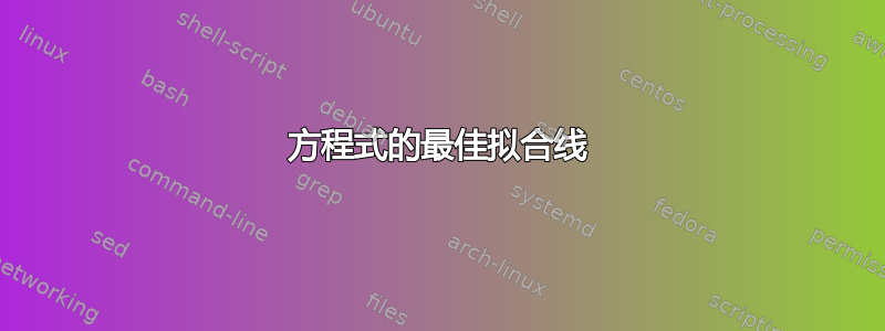
\conductivity这符合您的需求吗?我使用命令将每个电压的回归线值添加到表中\pgfplotstablecreatecol。然后,您可以轻松地在图中使用这些值,或者使用它pgfplotstable为您提供包含这些值的表格。
\documentclass[]{article}
\usepackage{filecontents,pgfplots}
\usepackage{pgfplotstable}
% recommended:
\usepackage{booktabs}
\usepackage{array}
\usepackage{colortbl}
%\usepgfplotslibrary{clickable}
\pgfdeclareplotmark{halfcircle}{%
\begin{pgfscope}
\pgfsetfillcolor{white}%
\pgfpathcircle{\pgfpoint{0pt}{0pt}}
{\pgfplotmarksize}
\pgfusepathqfillstroke
\end{pgfscope}%
\pgfpathmoveto
{\pgfpoint{\pgfplotmarksize}{0pt}}
\pgfpatharc{0}{180}{\pgfplotmarksize}
\pgfpathclose
\pgfusepathqfill
}

\begin{filecontents}{conductivity.dat}
L(cm)   50mA    100mA  200mA 400mA 800mA 1000mA
0.0000  0.0000 0.0000 0.000 0.000 0.000 0.000
2.0000  0.0342 0.0635 0.128 0.260 0.520 0.650
3.0000  0.0555 0.1043 0.212 0.423 0.840 1.030
4.0000  0.1104 0.2064 0.396 0.809 1.300 1.700
6.0000  0.1350 0.2426 0.502 1.034 2.010 2.471
7.0000  0.1669 0.3326 0.673 1.339 2.610 3.140

\end{filecontents}

\begin{document}
\pgfplotstableread{conductivity.dat}{\conductivity}
% create the `regression' columns:
\pgfplotstablecreatecol[linear regression={y=50mA}]{regression 50mA}{\conductivity}
\pgfplotstablecreatecol[linear regression={y=100mA}]{regression 100mA}{\conductivity}
\pgfplotstablecreatecol[linear regression={y=200mA}]{regression 200mA}{\conductivity}
\pgfplotstablecreatecol[linear regression={y=400mA}]{regression 400mA}{\conductivity}
\pgfplotstablecreatecol[linear regression={y=800mA}]{regression 800mA}{\conductivity}
\pgfplotstablecreatecol[linear regression={y=1000mA}]{regression 1000mA}{\conductivity}

\centering
\begin{tikzpicture}[scale=1]
\begin{axis}[xmin = 0, ymin = 0,
            xlabel=Bed depth (cm),
            ylabel = Voltage,
            width=1.2\textwidth,
            height=0.8\textwidth, legend pos={north west},
            xticklabel style={/pgf/number format/1000 sep=}]
% regression
\addplot[black, no markers] table [x={L(cm)}, y={regression 50mA}] {\conductivity};\addlegendentry{50mA}
\addplot[orange, no markers] table [x={L(cm)}, y={regression 100mA}] {\conductivity};\addlegendentry{100mA}
\addplot[magenta, no markers] table [x={L(cm)}, y={regression 200mA}] {\conductivity};\addlegendentry{200mA}
\addplot[green, no markers] table [x={L(cm)}, y={regression 400mA}] {\conductivity};\addlegendentry{400mA}
\addplot[blue, no markers] table [x={L(cm)}, y={regression 800mA}] {\conductivity};\addlegendentry{800mA}
\addplot[red, no markers] table [x={L(cm)}, y={regression 1000mA}] {\conductivity};\addlegendentry{1000mA}
% data
\addplot+[only marks][black, mark = otimes] table [x={L(cm)}, y={50mA}] {\conductivity};\addlegendentry{50mA}
\addplot+[only marks] [mark = star, black] table [x={L(cm)}, y={100mA}] {\conductivity};\addlegendentry{100mA}
\addplot+[only marks] [mark = o, black ] table [x={L(cm)}, y={200mA}] {\conductivity};\addlegendentry{200mA}
\addplot+[only marks] [mark = +, black] table [x={L(cm)}, y={400mA}] {\conductivity};\addlegendentry{400mA}
\addplot+[only marks] [mark = oplus, black] table [x={L(cm)}, y={800mA}] {\conductivity};\addlegendentry{800mA}
\addplot+[only marks] [mark=halfcircle, black] table [x={L(cm)}, y={1000mA}] {\conductivity};\addlegendentry{1000mA}
\end{axis}
\end{tikzpicture}

\pgfplotstabletypeset[columns={50mA, 100mA, 200mA, 400mA, 800mA, 1000mA}]\conductivity\\

\pgfplotstabletypeset[columns={regression 50mA, regression 100mA, regression 200mA, regression 400mA, regression 800mA}]\conductivity
\end{document}