

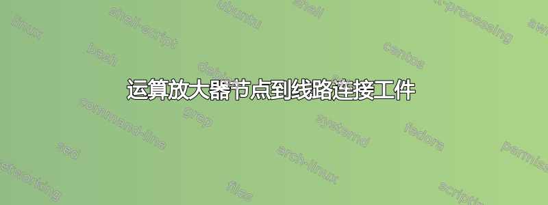
我对运算放大器节点和连接它的线路之间的连接有轻微的视觉干扰。

也许情况并没有好转,或者我需要调整一些线条粗细?谢谢你的帮助!
\begin{figure}[!htbp]
\centering
\ctikzset{voltage/distance from node=.2}% defines arrow's distance from nodes
\ctikzset{voltage/distance from line=.02}% defines arrow's distance from wires
\ctikzset{voltage/bump b/.initial=.1}% defines arrow's curvature
\begin{tikzpicture}

\draw
(0,0) node[ocirc] (A) {}
(0,3) node [ocirc] (B) {}
(11,0) node[ocirc] (C) {}
(11,3.5) node[ocirc] (D) {}
(3,3) node[circ] (E) {}
(6,3) node[circ] (F) {}
(10,3.5) node[circ] (O) {}
(10,5) node[circ] (OT) {}
(8,3.5) node[op amp] (opamp) {}

(B) to [open,v=$u_e(t)$] (A)
(D) to [open, v^=$u_a(t)$] (C)

(A) -- (C)

(B) to[R, l=$R_1$] (E) to[R,l=$R_2$] (opamp.+)
(F) to[C,l=$C_1$] (6,0)

(E) -- (3,6) to[C, l=$C_2$] (10,6) -- (O) -- (opamp.out)
(opamp.-) -- (6,4) -- (6,5) -- (OT)
(O) -- (D)
(opamp.+) node[left] {}
(opamp.-) node[left] {}
(opamp.out) node[right] {}
;
\end{tikzpicture}
\caption{2nd Order Low Pass}
\label{fig:lowpass}
\结束{图}
答案1
您必须调整坐标,opamp.-不完全位于 y = 4,因此该线不是水平的。为了避免显式的 xy 坐标,您可以这样做
(opamp.-) -- (opamp.- -| F) |- (OT)
-|/语法|-描述如下TikZ:箭头的 |- 符号到底起什么作用?
另一个也一样,你需要以某种方式确保F和opamp.+位于相同的 y 坐标。一种做法是设置不同的图表,F相对于放置opamp,而不是使用明确的坐标。如果你愿意,你可以将所有内容相对于其他内容放置,例如:
\documentclass[border=5mm,tikz]{standalone}
\usepackage{circuitikz}
\usetikzlibrary{positioning}
\begin{document}

\ctikzset{voltage/distance from node=.2}% defines arrow's distance from nodes
\ctikzset{voltage/distance from line=.02}% defines arrow's distance from wires
\ctikzset{voltage/bump b/.initial=.1}% defines arrow's curvature

\begin{tikzpicture}

\draw
  node[op amp] (opamp) {}
  node[circ, right=of opamp] (O) {}
  node[circ, left=of opamp.+] (F) {}
  node[ocirc, right=of O,label=right:D] (D) {}
  node[circ, left=3cm of F] (E) {}
  node[circ, above=of O] (OT) {}
  node[ocirc,left=3cm of E] (B) {}
  node[ocirc, below=3cm of B] (A) {}
  (A -| D) node[ocirc] (C) {}
  % define a few helper coordinates, used below when drawing the connections
  (F |- A) coordinate (tmpC1)
  coordinate[above=of OT] (tmpC2)
  coordinate[left=of opamp.-] (tmpF)

(B) to [open,v=$u_e(t)$] (A)
(D) to [open, v^=$u_a(t)$] (C)

(A) -- (C)

(B) to[R, l=$R_1$] (E) to[R,l=$R_2$] (opamp.+)
(F) to[C,l=$C_1$] (tmpC1)

(E) -- (E |- tmpC2) to[C, l=$C_2$] (tmpC2) -- (O) -- (opamp.out)
(opamp.-) -- (tmpF) |- (OT)
(O) -- (D)
(opamp.+) node[left] {}
(opamp.-) node[left] {}
(opamp.out) node[right] {}
;
\end{tikzpicture}
\end{document}
答案2
这Torbjørn T. 的回答是正确的,但还要注意 PDF 查看器可以发挥作用。不同的抗锯齿算法可以显示不同的东西。例如,使用 Torbjørn 的代码,在相同的缩放比例(150%)下,您可以看到:
- 在
okular(这对于其他事情来说很棒,但是......请注意线路和电容器)

- 在
evince(我无法使用vimtex反向引用,尽管在我的显示器上呈现效果更好)...
