

我已经为我的框图编写了代码,如下所示:

\documentclass[10pt]{article}
\usepackage{adjustbox}
\usepackage{tikz}
\usetikzlibrary{plotmarks,matrix,decorations.pathreplacing,arrows.meta,calc,chains,shapes.geometric,backgrounds,fit,arrows,positioning}

\tikzset{
block/.style={
  draw,
  fill=blue!20,
  rectangle,
  minimum height=5em,
  minimum width=6em
  },
  every label/.append style = {text= blue, align=center},
  blockk/.style={
  draw,
  fill=blue!20,
  rectangle,
  minimum height=2.5em,
  minimum width=2.5em
  },
   blockkk/.style={
  draw,
  fill=blue!20,
  rectangle,
  minimum height=11.3em,
  minimum width=14em
  },
sum/.style={
  draw,
  fill=blue!20,
  circle,
  minimum size=0.5cm,
  },
input/.style={coordinate},
output/.style={coordinate},
pinstyle/.style={pin edge={to-,thin,black}}
}

\begin{document}
\begin{figure*}
\begin{adjustbox}{width=\textwidth,height=\textheight,keepaspectratio}
\begin{tikzpicture}[auto,>=latex']
    % We start by placing the blocks
    \node [input, name=input] {};
    \node [sum, right = of input] (sum) {};
    \node [blockk, above right = of sum] (derivative) {$D_t^p$};
    \node [blockk, below = 0.25cm of derivative] (integral) {$D_t^{-p}$};
    \node [blockkk, below right = -0.8cm and 1.2cm of derivative] (controller) {Predictive GT2-FLC};
    \node [sum, right = 2cm of controller] (sum1) {\tiny+};
    \node [block, right = 2cm of sum1] (system) {System};
    \node [block, below = 2cm of sum1] (compensator) {Compensator};
    \node [block, above right = 2cm and -2.1cm of system] (estimator) {IT2-FLS Based Model Estimator};
    \node [sum, below right = 1cm and 2.1cm of estimator] (sum2) {};
    \node[above=-2pt] at (sum.center){\tiny $+$};
    \node[below=-2pt] at (sum.center){\tiny $-$};
    \node[above=-2pt] at (sum2.center){\tiny $+$};
    \node[below=-2pt] at (sum2.center){\tiny $-$};

    \draw [draw,->] (input) -- node {\textcolor{blue}{\Large $z_d$}} (sum); %input
    \draw [draw,->] (sum) -- node {\textcolor{blue}{\Large $e$}} (+2cm,0)--(+2cm,+1.6cm)--(derivative); %derivative
    \draw [draw,->] (+2cm,0.5)--(integral); % e to integral
    \draw [draw,->] (derivative) -- (4.55,1.6); %integral to controller
    \draw [draw,->] (integral) -- (4.55,0.5);%derivative to controller
    \draw [draw,->] (2,-0.6)--(4.55,-0.6); %e to controller
    \draw[double,dashed,-](sum2)--(21,1.7)-- ([yshift=-1em]estimator.south east) -- ([yshift=1em]estimator.north west)--node[above]{\textcolor{blue}{\large Learning by adaptation law}}(9.5,5);
    \draw [draw,->] (controller) -- node {\textcolor{blue}{\Large $u_c$}} (sum1); %controller to sum1
    \draw [draw,->] (compensator) -- node {\textcolor{blue}{\Large $u_{cpr}$}} (sum1); %sum1 to compensator
    \draw [draw,->] (+2cm,0.5)--(+2,-3.3)--(compensator);%e to compensator
    \draw [draw,->] (sum1) -- node {\textcolor{blue}{\Large $u$}} (system); %sum1 to system
    \draw [draw,->] (12.5,-0)--(12.5,4.2)--(14.1,4.2); %u to estimator
    \draw [draw,<->] (4.55,-1.7)->(3,-1.7)--(3,-5)--(16.5,-5)--(16.5,1.5)--(13.5,1.5)--(13.5,3.3)->(14.1,3.3); %controller to estimator
    \draw [draw,->] (estimator) -- (+16.7cm,6)--node[above]{\textcolor{blue}{\large Fractional-order Fuzzy Model}}(7,6)--(controller); %estimator to controller
    \draw [draw,->] (estimator)--node {\textcolor{blue}{\Large $\hat{z}$}} (21.7,3.75)--(sum2); %estimator to sum2
    \draw [draw,->] (21.7,3.75)--(23.7,3.75)--(23.7,-6)--(1.25,-6)--(sum); %yhat to sum
    \draw [draw,->] (system)-- node {\textcolor{blue}{\Large $z$}} (21.7,0)-- (sum2); %system to sum2
    \draw [draw,->] (sum2) --(22.7,1.7)--(22.7,-3.3)--node[above]{\textcolor{blue}{\Large $\hat{e}$}} (compensator); %sum2 to compensator
    \draw[double,dashed,-] ([yshift=-1em]controller.south east) -- ([yshift=1em]controller.north west)--node[above] {\textcolor{blue}{\large Learning by BBO}}(1.4,2.35);

\end{tikzpicture}
\end{adjustbox}
\end{figure*}
\end{document}
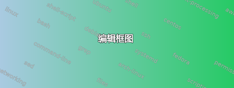
现在,我想做一些更改,如下图箭头所示:

箭头 1- 使其看起来如图所示,完全通过编码完成
箭头 2- 使其看起来如图所示,完全通过编码完成
箭头 3- 使其看起来如使用图像所示。使用任意 120*120(像素)图像
答案1
其他东西周围的矩形可以通过矩阵实现(除非您需要以某种形状或形式变换这个矩形)。
随着generate anchors来自最近答案的解决方案我们在每个节点的左侧创建一堆锚点,我们可以用它来引用其他节点的位置或将线连接到它。
该ext.paths.ortho库提供了各种正交连接,ext.positioning-plus使得查找参考多个其他节点的坐标变得更容易一些。
我提供了一张subtitle图,其中一条粗线和一个节点位于其他东西下方。我不确定这条线应该有多长,因为在你的草图中,它有时比上面的线长,有时比上面的线短。
代码
\documentclass[tikz]{standalone}
\usetikzlibrary{arrows.meta, calc, ext.paths.ortho, ext.positioning-plus, graphs, quotes}
\makeatletter
\pgfset{
  @generate anchors/.code n args={4}{%
    \pgfmathloop\pgfmathparse{\pgfmathcounter/(#2+1)}%
      \pgfset{generate anchors/.expanded={#1 \pgfmathcounter/#2:\pgfmathresult}{#3}{#4}}%
      \ifnum\pgfmathcounter<#2\relax\repeatpgfmathloop},
  @generate anchor/.code args={#1:#2:#3:#4}{%
    \pgfdeclaregenericanchor{#1}{%
      \pgfpointlineattime{#2}{\pgf@sh@reanchor{##1}{#3}}{\pgf@sh@reanchor{##1}{#4}}}},
  generate anchors/.style n args={3}{
    /utils/tempa/.style={/pgf/@generate anchor={##1:#2:#3}}, /utils/tempa/.list={#1}}}
\makeatother
\pgfset{@generate anchors={in}{8}{north west}{south west}}
\tikzset{
  subtitle length/.initial=2cm,
  subtitle/.pic={
    \coordinate[below={.6666em of #1}] (@);
    \draw[shift=(@), ultra thick, pic actions] (left:\pgfkeysvalueof{/tikz/subtitle length})
                                           -- (right:\pgfkeysvalueof{/tikz/subtitle length})
      node[below, midway, node font=\Large, style/.expand once=\tikzpictextoptions]{\tikzpictext};},
  /utils/temp/.style n args={3}{% allow r-du, r-ud, r-lr, r-rl to be used inside to and edges
    #1#2/.style={to path={r-#1#2(\tikztotarget)\tikztonodes}},
    #1#2 through point/.style={to path={% udlr paths through a point
      let \p{start}=($(##1)-(\tikztostart)$), \p{target}=($(##1)-(\tikztotarget)$) in
      r-#1#2[#1#2 distance/.expanded={min(abs(#3{start}),abs(#3{target}))}, from center]
      (\tikztotarget)\tikztonodes}}},
  /utils/temp/.list={lr\x, rl\x, du\y, ud\y}}
\begin{document}
\begin{tikzpicture}[
  Block/.style args={#1x#2}{
    draw, fill=blue!20, shape=rectangle, align=center, minimum width={#1}, minimum height={#2}},
  block/.style ={Block =  0pt   x  0pt},
  block1/.style={Block =  6em   x  5em},
  block2/.style={Block =  2.5em x  2.5em},
  block3/.style={Block = 14em   x 11.3em},
  every edge quotes/.append style = {text=blue, align=center},
  sum/.style={
    draw, fill=blue!20, circle, minimum size=0.5cm, align=center, node font=\tiny},
  input/.style={coordinate},
%  output/.style={coordinate},
  auto, >=Latex, node distance=\nd, ortho/install shortcuts,
  up and down curve/.style={insert path={
      (0,0) coordinate (curve-start)
            to[out=30, in=180, in distance=3mm] ++(1, 2) -- ++(right:.5)
            to[out= 0, in=150, out distance=3mm] ++(1,-2)
         #1 ++(left:.2) coordinate (curve-end) [rounded corners]
            to[out=180, in=-80] ++(-1.05, 1.7) [sharp corners]
            to[out=260, in=0] (right:.2)}}
]
\newcommand*\nd{1cm}

\node [input] (input) {};
\node [sum, right = of input] (sum) {$+$\\$-$};
\matrix[fill=teal!50, draw, right=3:of sum] (controller){
  \node[block] (c1) {Learning by\\BBO}
   node[block, below=of c1, xshift=1.5cm] (c2) {Prediction\\Model};
  \path[horizontal vertical, ->] (c1) edge (c2) (c2) edge (c1);
  \pic["MPC"] {subtitle=(c1)(c2)};
\\};
\node [block2, left = of controller.in 1/8] (derivative) {$D_t^p$}
  edge[-*, ->] (controller);
\node [block2, left = of controller.in 4/8] (integral) {$D_t^{-p}$}
  edge[-*, ->] (controller);
\node[sum, right=1.5:of controller] (sum1) {$+$};
\node[block1, below=1.5:of sum1] (compensator) {Compensator};
\matrix[block, right=2:of sum1] (system) {
  \node[inner sep=+0pt](c1){\includegraphics[width=2cm, keepaspectratio]{example-image}};
  \pic["Model", subtitle length=1.2cm] {subtitle=(c1)};
\\};
\matrix[block, west above=of system] (estimator){
  \foreach[count=\i from -1] \c in {blue, orange, green}
    \fill[\c, opacity=.5, shift=(right:\i), name suffix=\i, up and down curve=--] -- cycle;
  \foreach \i in {-1, 0, 1}
    \draw[shift=(right:\i), up and down curve=];
  \pic["Type "]{subtitle=(curve-start-1)(curve-end1)};
\\};
\node[sum, right=of estimator.south east] (sum2) {$+$\\$-$};

\coordinate[below=.5:of compensator] (comp1);
\coordinate[below=.5:of comp1]       (comp2);
\coordinate[right=of sum2]           (sum21);
\graph[use existing nodes] {
  input ->["$Z_d$"] sum
        ->[-|-, /tikz/ortho/distance=\nd/2] {
          derivative, integral, compensator, controller[> {"$e$" very near start, graphs/right anchor=in 6/8}]},
  controller ->["$u_c$"] sum1
             ->["$u$"] system
             ->["$z$" near start, -|] sum2
             ->["$\hat e$" very near end, rl] compensator
             ->["$u_{\mathrm{epr}}$"] sum1
             ->[-|-, /tikz/ortho/ratio=.25, right anchor=in 3/8] estimator
             ->["$\hat z$" near start, -|] sum2,
  estimator ->[ud, clear >, "Fractional-order Fuzzy Model"'] controller,
  estimator ->[left anchor=in 5/8, right anchor=in 8/8, to path={
    --++(left:\nd/2) {to[du through point=comp1] ([shift=(left:\nd/2)]\tikztotarget)} -- (\tikztotarget)}] controller,
  estimator ->[to path={-| (sum21) |- (comp2) -| (\tikztotarget)}] sum
};
\end{tikzpicture}
\end{document}
输出

答案2
这里有一些方法可以实现。
一般的:
- 对于开发来说它更容易使用
standalone - 这里不需要so
\figure和adjustbox - 软件包
graphicx允许您包含图像
保存为icon.png:

箭头 3 的主要思想:
- 视为节点内的 LaTeX 文本
{ } - 所以
\includegraphics - 用于
\\新线,以及align=center - 用于
\hrulefill规则
箭头 1 的主要思想:
- 引入了
pic-style命名的mpcvia\tikzset{} - 它手动放置框、线和文本(就我而言,是通过眼睛)
- 像调用节点一样调用
\pic {};,指定样式为{mpc}; \pics放置任意数量的- 因为 node-text 接受 LaTeX 里面的
{},{\tikz{..};};是一个有效的参数 - 最简单的方法是在所述节点中设置填充颜色
- 你也可以缩放图片,但你需要检查变换选项以避免......好吧,你会看到
箭 2 ...
您可以用类似的方法构建。寻找cycle闭合路径的方法。在手册中寻找弯曲线性线条的方法。寻找重叠部分的透明度。
考虑到这一点,您应该能够调整您的绘图。

%\documentclass[10pt]{article}
\documentclass[10pt,border=3mm,tikz]{standalone}% better for development
%\usepackage{adjustbox}% then this one is not needed
\usepackage{tikz}
\usetikzlibrary{plotmarks,matrix,decorations.pathreplacing,
                arrows.meta,calc,chains,shapes.geometric,
                backgrounds,fit,arrows,positioning}
\usepackage{graphicx}% for the image

\tikzset{
block/.style={
  draw,
  fill=blue!20,
  rectangle,
  minimum height=5em,
  minimum width=6em
  },
every label/.append style = {text= blue, align=center},
blockk/.style={
  draw,
  fill=blue!20,
  rectangle,
  minimum height=2.5em,
  minimum width=2.5em
  },
blockkk/.style={
  draw,
  fill=blue!20,
  rectangle,
  minimum height=11.3em,
  minimum width=14em
  },
sum/.style={
  draw,
  fill=blue!20,
  circle,
  minimum size=0.5cm,
  },
input/.style={coordinate},
output/.style={coordinate},
pinstyle/.style={pin edge={to-,thin,black}}
}

\begin{document}

% ~~~ arrow 3 ~~~~~~~~~~~~~~~~~~~~~~~~~~~~~~~~
\begin{tikzpicture}
    \node[align=center,% for multiline
          font={\Large\bfseries},% if you want larger fonts; the old bold-definition works
          fill=blue!20,% background; make image transparent with a paint program, if needed
          draw,
    ]
            {\includegraphics[scale=1]{icon}\\
            \hrulefill\\
            Model};
\end{tikzpicture}


% ~~~ arrow 1 ~~~~~~~~~~~~~~~~~~~~~~~~~~~~~~~~
\tikzset{
    bx/.style={align=center, draw, fill=blue!20},
    > = {Stealth},
    tx/.style={font={\Large\bfseries\sf}},% if you prefer san serif
    %
    mpc/.pic={
        % ~~~ blocks ~~~~~~~~~~~~~~~~
        \node[bx] (A)               {Learning by\\XY()};
        \node[bx] (B) at (1.5,-1.5) {Prediction\\Model)};
        % ~~~ connectors ~~~~~~~~~~~~~~
        \draw [->] (A.east) -| (B.45);% anchor point in polar coordinates
        \draw [->] (B.west) -| (A.220);
        % ~~~ rest ~~~~~~~~~~~~
        \node[tx] at (0.9,-3) {MPC};
        \draw[line width=3pt] (-1,-2.5) -- +(3.8,0);% relative move
    }
}
% ~~~ now using said pic ~~~~~~~~~~
\begin{tikzpicture}
    \pic {mpc}; % place like nodes; type of pic inside the { }
    \pic at (5,0) {mpc};
    \node[draw,fill=yellow] at (0,-6) {\tikz{\pic {mpc};}};% LaTeX inside { }
\end{tikzpicture}


%\begin{figure*}
%\begin{adjustbox}{width=\textwidth,height=\textheight,keepaspectratio}
\begin{tikzpicture}[auto,>=latex']
    % We start by placing the blocks
    \node [input, name=input] {};
    \node [sum, right = of input]                                   (sum) {};
    \node [blockk, above right = of sum]                            (derivative) {$D_t^p$};
    \node [blockk, below = 0.25cm of derivative]                    (integral) {$D_t^{-p}$};
    \node [blockkk, below right = -0.8cm and 1.2cm of derivative]   (controller) {Predictive GT2-FLC};
    \node [sum, right = 2cm of controller]                          (sum1) {\tiny+};
    \node [block, right = 2cm of sum1] (system)                     {System};
    \node [block, below = 2cm of sum1]                              (compensator) {Compensator};
    \node [block, above right = 2cm and -2.1cm of system]           (estimator) {IT2-FLS Based Model Estimator};
    \node [sum, below right = 1cm and 2.1cm of estimator]           (sum2) {};
    \node[above=-2pt] at            (sum.center){\tiny $+$};
    \node[below=-2pt] at            (sum.center){\tiny $-$};
    \node[above=-2pt] at            (sum2.center){\tiny $+$};
    \node[below=-2pt] at            (sum2.center){\tiny $-$};

    % ~~~ connections ~~~~~~~~~~~~~~~~~~~~~~~~~~~~~~~~~~~~~~~~~~~~~~~~~
    \draw [draw,->] (input) -- node {\textcolor{blue}{\Large $z_d$}} (sum); %input
    \draw [draw,->] (sum) -- node {\textcolor{blue}{\Large $e$}} (+2cm,0)--(+2cm,+1.6cm)--(derivative); %derivative
    \draw [draw,->] (+2cm,0.5)--(integral); % e to integral
    \draw [draw,->] (derivative) -- (4.55,1.6); %integral to controller
    \draw [draw,->] (integral) -- (4.55,0.5);%derivative to controller
    \draw [draw,->] (2,-0.6)--(4.55,-0.6); %e to controller
    \draw[double,dashed,-](sum2)--(21,1.7)-- ([yshift=-1em]estimator.south east) -- ([yshift=1em]estimator.north west)--node[above]{\textcolor{blue}{\large Learning by adaptation law}}(9.5,5);
    \draw [draw,->] (controller) -- node {\textcolor{blue}{\Large $u_c$}} (sum1); %controller to sum1
    \draw [draw,->] (compensator) -- node {\textcolor{blue}{\Large $u_{cpr}$}} (sum1); %sum1 to compensator
    \draw [draw,->] (+2cm,0.5)--(+2,-3.3)--(compensator);%e to compensator
    \draw [draw,->] (sum1) -- node {\textcolor{blue}{\Large $u$}} (system); %sum1 to system
    \draw [draw,->] (12.5,-0)--(12.5,4.2)--(14.1,4.2); %u to estimator
    \draw [draw,<->] (4.55,-1.7)->(3,-1.7)--(3,-5)--(16.5,-5)--(16.5,1.5)--(13.5,1.5)--(13.5,3.3)->(14.1,3.3); %controller to estimator
    \draw [draw,->] (estimator) -- (+16.7cm,6)--node[above]{\textcolor{blue}{\large Fractional-order Fuzzy Model}}(7,6)--(controller); %estimator to controller
    \draw [draw,->] (estimator)--node {\textcolor{blue}{\Large $\hat{z}$}} (21.7,3.75)--(sum2); %estimator to sum2
    \draw [draw,->] (21.7,3.75)--(23.7,3.75)--(23.7,-6)--(1.25,-6)--(sum); %yhat to sum
    \draw [draw,->] (system)-- node {\textcolor{blue}{\Large $z$}} (21.7,0)-- (sum2); %system to sum2
    \draw [draw,->] (sum2) --(22.7,1.7)--(22.7,-3.3)--node[above]{\textcolor{blue}{\Large $\hat{e}$}} (compensator); %sum2 to compensator
    \draw[double,dashed,-] ([yshift=-1em]controller.south east) -- ([yshift=1em]controller.north west)--node[above] {\textcolor{blue}{\large Learning by BBO}}(1.4,2.35);

\end{tikzpicture}
%\end{adjustbox}
%\end{figure*}
\end{document}