

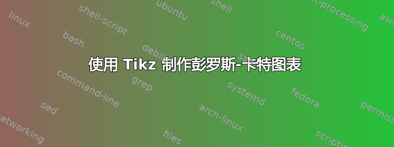
我正在尝试绘制史瓦西背景中粒子运动的彭罗斯图。我能够绘制该图,感谢本文由 Izaak Neutelings 撰写 代码如下:
% Author: Izaak Neutelings (September 2021)
% Inspiration:
%   https://jila.colorado.edu/~ajsh/insidebh/penrose.html
%   https://tex.stackexchange.com/questions/99124/how-to-draw-penrose-diagrams-with-tikz
%   coordinates: https://arxiv.org/pdf/physics/0611033.pdf
%   https://arxiv.org/pdf/0711.0873.pdf
\documentclass[border=3pt,tikz]{standalone}
\usepackage{tikz}
\usepackage{amsmath} % for \text
\usepackage{mathrsfs} % for \mathscr
\usepackage{xfp} % higher precision (16 digits?)
\usepackage[outline]{contour} % glow around text
\usetikzlibrary{decorations.markings,decorations.pathmorphing}
\usetikzlibrary{angles,quotes} % for pic (angle labels)
\usetikzlibrary{arrows.meta} % for arrow size
\contourlength{1.4pt}

\newcommand{\calI}{\mathscr{I}} %\mathcal
\tikzset{>=latex} % for LaTeX arrow head
\colorlet{myred}{red!80!black}
\colorlet{myblue}{blue!80!black}
\colorlet{mygreen}{green!80!black}
\colorlet{mydarkred}{red!50!black}
\colorlet{mydarkblue}{blue!50!black}
\colorlet{mylightblue}{mydarkblue!6}
\colorlet{mypurple}{blue!40!red!80!black}
\colorlet{mydarkpurple}{blue!40!red!50!black}
\colorlet{mylightpurple}{mydarkpurple!80!red!6}
\colorlet{myorange}{orange!40!yellow!95!black}
\tikzstyle{cone}=[mydarkblue,line width=0.2,top color=blue!60!black!30,
                  bottom color=blue!60!black!50!red!30,shading angle=60,fill opacity=0.9]
\tikzstyle{cone back}=[mydarkblue,line width=0.1,dash pattern=on 1pt off 1pt]
\tikzstyle{world line}=[myblue!60,line width=0.4]
\tikzstyle{world line t}=[mypurple!60,line width=0.4]
\tikzstyle{particle}=[mygreen,line width=0.5]
\tikzstyle{photon}=[-{Latex[length=4,width=3]},myorange,line width=0.4,decorate,
                    decoration={snake,amplitude=0.9,segment length=4,post length=3.8}]
\tikzstyle{singularity}=[myred,line width=0.6,decorate,
                         decoration={zigzag,amplitude=2,segment length=6.17}]
\tikzset{declare function={%
  penrose(\x,\c)  = {\fpeval{2/pi*atan( (sqrt((1+tan(\x)^2)^2+4*\c*\c*tan(\x)^2)-1-tan(\x)^2) /(2*\c*tan(\x)^2) )}};%
  penroseu(\x,\t) = {\fpeval{atan(\x+\t)/pi+atan(\x-\t)/pi}};%
  penrosev(\x,\t) = {\fpeval{atan(\x+\t)/pi-atan(\x-\t)/pi}};%
  kruskal(\x,\c)  = {\fpeval{asin( \c*sin(2*\x) )*2/pi}};% Penrose coordinates for Kruskal
}}
\def\tick#1#2{\draw[thick] (#1) ++ (#2:0.04) --++ (#2-180:0.08)}
\def\Nsamples{20} % number samples in plot

% LIGHTCONE
\def\R{0.08} % size lightcone
\def\e{0.08} % vertical scale
\def\ang{45} % angle light cone
\def\angb{acos(sqrt(\e)*sin(\ang))} % angle ellipse center to point of tangency
\def\a{\R*sin(\ang)*sqrt(1-\e*sin(\ang)^2)/(1-\e*sin(\ang)^2)} % vertical radius
\def\b{\R*sqrt(\e)*sin(\ang)*cos(\ang)/(1-\e*sin(\ang)^2)} % horizontal radius
\def\coneback#1{ % light cone part to be drawn behind world lines
  \draw[cone back] % dashed line back
    (#1)++(-45:\R) arc({90-\angb}:{90+\angb}:{\a} and {\b});
  \draw[cone,shading angle=-60] % top edge & inside
    (#1)++(0,{\R*cos(\ang)/(1-\e*sin(\ang)^2)}) ellipse({\a} and {\b});
}
\def\conefront#1{ % light cone part to be drawn over world lines
  \draw[cone] % light cone outside
    (#1) --++ (45:\R) arc({\angb-90}:{-90-\angb}:{\a} and {\b})
     --++ (-45:2*\R) arc({90-\angb}:{-270+\angb}:{\a} and {\b}) -- cycle;
}

\begin{document}
\begin{tikzpicture}[scale=3.2]
  \message{Extended Penrose diagram: Schwarzschild black hole^^J}

  \def\R{0.08} % size lightcone
  \def\Nlines{3} % number of world lines (at constant r/t)
  \pgfmathsetmacro\ta{1/sin(90*1/(\Nlines+1))} % constant r/t value 1
  \pgfmathsetmacro\tb{sin(90*2/(\Nlines+1))}   % constant r/t value 2
  \pgfmathsetmacro\tc{1/sin(90*2/(\Nlines+1))} % constant r/t value 3
  \pgfmathsetmacro\td{sin(90*1/(\Nlines+1))}   % constant r/t value 4
  \coordinate (-O) at (-1, 0); % center III: origin (r,t) = (0,0)
  \coordinate (-N) at (-1, 1); % north III: t=+infty, i+
  \coordinate (O)  at ( 1, 0); % center I: origin (r,t) = (0,0)
  \coordinate (S)  at ( 1,-1); % south I: t=-infty, i-
  \coordinate (N)  at ( 1, 1); % north I: t=+infty, i+
  \coordinate (E)  at ( 2, 0); % east I:  r=-infty, i0
  \coordinate (W)  at ( 0, 0); % west I:  r=+infty, i0
  \coordinate (B)  at ( 0,-1); % singularity bottom
  \coordinate (X0) at ({asin(sqrt((\ta^2-1)/(\ta^2-\tb^2)))/90},
                       {-acos(\ta*sqrt((1-\tb^2)/(\ta^2-\tb^2)))/90}); % particle 1
  \coordinate (X1) at ({asin(sqrt((\tc^2-1)/(\tc^2-\td^2)))/90},
                       {acos(\tc*sqrt((1-\td^2)/(\tc^2-\td^2)))/90}); % particle 2
  \coordinate (X2) at (45:0.87); % particle falling in BH horizon
  \coordinate (X3) at (0.60,1.05); % particle falling in BH singularity

  % AXES
  \draw[->,thick] (0,-0.1) -- (0,1.15) node[above=1,left=-1] {$v$};
  \draw[->,thick] (-0.1,0) -- (2.15,0) node[left=1,above=0] {$u$};

  \begin{scope}

    % CLIP to fill inside zigzag lines
    \clip[decorate,decoration={zigzag,amplitude=2,segment length=6.17}]
      (-N) -- (N) --++ (1.1,0.1) |-++ (-3.1,-2.3) -- cycle;

    % REGIONS FILLS
    \fill[mylightpurple] (-N) |-++ (2,0.1) -- (N) -- (W) -- cycle;
    \fill[mylightblue] (N) -- (E) -- (S) -- (W) -- cycle;


    % WORLD LINES
    \draw[world line] (N) -- (S);
    \draw[world line t] (W) -- (E) (W) -- (0,1.1);
    \message{Making world lines...^^J}
    \foreach \i [evaluate={\c=\i/(\Nlines+1); \cs=sin(90*\c);}] in {1,...,\Nlines}{
      \message{  Running i/N=\i/\Nlines, c=\c, cs=\cs...^^J}
      \draw[world line t,samples=\Nsamples,smooth,variable=\x,domain=0:2] % region I, constant t
        plot(\x,{-kruskal(\x*pi/4,\cs)})
        plot(\x,{ kruskal(\x*pi/4,\cs)});
      \draw[world line,samples=\Nsamples,smooth,variable=\y,domain=0:2] % region I, constant r
        plot({1-kruskal(\y*pi/4,\cs)},\y-1)
        plot({1+kruskal(\y*pi/4,\cs)},\y-1);
      \draw[world line,samples=\Nsamples,smooth,variable=\x,domain=0:2] % region II, constant r
        plot(\x-1,{1-kruskal(\x*pi/4,\cs)});
      \draw[world line t,samples=\Nsamples,smooth,variable=\y,domain=0:1.05] % region II constant t
        plot({-kruskal(\y*pi/4,\cs)},\y)
        plot({ kruskal(\y*pi/4,\cs)},\y);
    }

    % PARTICLE WORLD LINE
    \draw[particle]
      (S) to[out=77,in=-70] (X0) to[out=110,in=-80] (X1)
          to[out=100,in=-90] (X2) to[out=75,in=-80] (X3);

  \end{scope}


  % REGIONS
  \node[fill=mylightblue,inner sep=2] at (O) {I};
  \node[fill=mylightpurple,inner sep=2] at (0,0.64) {II};

  % BOUNDARIES
  \draw[singularity] (-N) -- node[pos=0.46,above left=-2] {\strut singularity} (N);
  \draw[singularity] (-N) -- node[pos=0.54,above right=-2] {\strut $r=0$} (N);
  \path (S) -- (W) node[mydarkblue,pos=0.50,below=-2.5,rotate=-45,scale=0.85]
    {anti-horizon $r=2GM$};
  \path (W) -- (N) node[mydarkblue,pos=0.32,above=-2.5,rotate=45,scale=0.85]
    {\contour{mylightpurple}{horizon $r=2GM$}};
  \draw[thick,mydarkblue] (N) -- (E) -- (S) --  (W) -- cycle;
  \draw[thick,mydarkblue] (W) -- (-N);

  % TICKS
  \node[below left=-1] at (W) {$0$};
  \tick{E}{90} node[right=4,below=-3] {$\pi/2$};
  \tick{S}{0} node[left=-1] {$-\pi/2$};
  \tick{N}{180} node[right=-1] {$\pi/2$};

  % INFINITY LABELS
  \node[above=1,right=1,mydarkblue] at (2.15,0) {$i^0$};
  \node[right=1,below=1,mydarkpurple] at (S) {$i^-$};
  \node[right=1,above=1,mydarkpurple] at (N) {$i^+$};
  \node[mydarkblue,above right=-1] at (1.5,0.5) {$\calI^+$};
  \node[mydarkblue,below right=-2] at (1.5,-0.5) {$\calI^-$};

\end{tikzpicture}

\end{document}
现在假设我有一个函数 T(R),我想绘制轨迹 (t=T, r=R)。我该如何将其绘制到上面的图表中?
举例来说,考虑 T(R) = R0 + sqrt(R)