

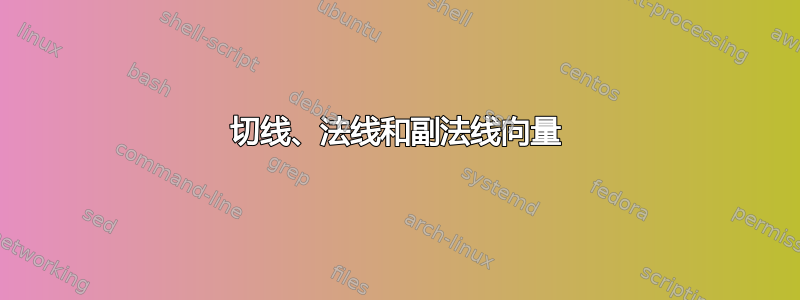
我想画一个示意图,说明笛卡尔坐标系和螺旋自然坐标系之间的坐标系关系。哪些工具(例如 tikz-3dplot、asymptote)更适合绘制这个?

答案1
我使用一些数学公式这里和Frenet–Serret 框架(或 TNB 框架)。

有了可用的公式,Asymptote 代码就变得简单明了。隐藏线可以是虚线,但我不喜欢这样,因为(T,N,B)那样也会是虚线 ^^

// http://asymptote.ualberta.ca/
unitsize(1cm);
import graph3;
currentprojection=orthographic(3,2,1.5,center=true,zoom=.9);
real a=2;
real h=8;
draw(scale(a,a,h)*unitcylinder,yellow+opacity(.3));
draw(Label("$x$",EndPoint,black),O--4X,gray,Arrow3());
draw(Label("$y$",EndPoint,black),O--4Y,gray,Arrow3());
draw(Label("$z$",EndPoint,black),O--10Z,gray,Arrow3());

triple r(real t){return (a*cos(t),a*sin(t),h*t/(2*pi));}
real tmin=0,tmax=2pi;
path3 g=graph(r,tmin,tmax,operator..);
draw(g,red+.6pt);

triple T(real t){return (-a*sin(t),a*cos(t),h/(2*pi));}
triple N(real t){return (-a*cos(t),-a*sin(t),0);}

pen pentan=purple;
pen pennor=red;
pen penbin=darkgreen;


real t=1;
triple P=r(t);
triple Pt=unit(T(t));         // the tangent vector at P
triple Pn=unit(N(t));         // the normal vector at P
triple Pb=cross(Pt,Pn);       // the binormal vector at P
draw(Label("$T$",EndPoint,pentan),P--P+Pt,pentan,Arrow3);
draw(Label("$N$",EndPoint,pennor),P--P+Pn,pennor,Arrow3);
draw(Label("$B$",EndPoint,penbin),P--P+Pb,penbin,Arrow3);

real s=3;
triple Q=r(s);
triple Qt=unit(T(s));         // the tangent vector at Q
triple Qn=unit(N(s));         // the normal vector at Q
triple Qb=cross(Qt,Qn);       // the binormal vector at Q
draw(Q--Q+Qt,pentan,Arrow3);
draw(Q--Q+Qn,pennor,Arrow3);
draw(Q--Q+Qb,penbin,Arrow3);

real c=4.3;
triple R=r(c);
triple Rt=unit(T(c));         // the tangent vector at R
triple Rn=unit(N(c));         // the normal vector at R
triple Rb=cross(Qt,Qn);       // the binormal vector at R
draw(R--R+Rt,pentan,Arrow3);
draw(R--R+Rn,pennor,Arrow3);
draw(R--R+Rb,penbin,Arrow3);
答案2
钛钾Z 解决方案。它使用3d和perspective库来避免一些三角计算。
我还创建了两个,\pic一个用于螺旋,另一个用于三个向量。这样我们就可以绘制其中任何一个,只需写出所涉及的角度即可。
代码:
\documentclass[tikz,border=1.618]{standalone}
\usetikzlibrary{3d,perspective}

\tikzset
{
  surface/.style={draw=cyan,left color=cyan,fill opacity=0.5},
  top/.style={draw=cyan,fill=cyan!30,fill opacity=0.5,canvas is xy plane at z=4},
  pics/helix/.style 2 args={code=% #1 = initial angle, #2 = final angle
    {\draw[pic actions] plot[domain=#1:#2,samples=0.5*#2-0.5*#1+1] ({cos(\x)},{sin(\x)},\x/180);}},
  pics/vectors/.style={code=% #1 = angle
    {\draw[green!50!black,-latex,opacity=0.3] ({cos(#1)},{sin(#1)},#1/180) -- ({0.4*cos(#1)},{0.4*sin(#1)},#1/180) node[pos=1.5] {$\vec N$};
     \begin{scope}[shift={({cos(#1)},{sin(#1)},#1/180)},rotate around z=90+#1,canvas is xz plane at y=0]
       \draw[blue!50!black,-latex]    (0,0) --++ ({atan(1/pi)}:0.75) node[pos=1.4] {$\vec T$};
       \draw[magenta!50!black,-latex] (0,0) --++ ({90+atan(1/pi)}:1) node[pos=1.3] {$\vec B$};
     \end{scope}}}
}

\begin{document}
\begin{tikzpicture}[isometric view,rotate around z=180,font=\small,
                    line cap=round,line join=round]
% axes
\draw[-latex] (0,0,0) -- (2,0,0) node[left]  {\strut$x$};
\draw[-latex] (0,0,0) -- (0,2,0) node[right] {\strut$y$};
% helix,   background
\pic[red] {helix={135}{315}};
\pic[red] {helix={495}{675}};
% z-axis,  background
\draw (0,0,0) -- (0,0,4);
% vectors, background
\foreach\i in {270,550}
  \pic {vectors=\i};
% cylinder
\draw[surface] (-45:1) arc (-45:135:1) --++ (0,0,4) arc (135:-45:1) -- cycle;
\draw[top] (0,0) circle (1);
% z-axis,  foreground
\draw[-latex] (0,0,4) -- (0,0,5.5) node[above] {$z$};
% helix,   foreground
\pic[red] {helix=  {0}{135}};
\pic[red] {helix={315}{495}};
\pic[red] {helix={675}{720}};
% vectors, foreground
\foreach\i in {30,110}
  \pic {vectors=\i};
\end{tikzpicture}
\end{document}
输出:
